I’ve written before about image similarity with pgvector and the usefulness of embeddings in geospatial workflows. The ability to represent observations as vectors gives us another way to search and compare data. With Earth observation embeddings, that comparison becomes geographic. I can start with a place and look for other places with similar characteristics.
Ai2’s October 22 release of OlmoEarth v1.3 provides an opportunity to try this with precomputed satellite embeddings. Its public announcement describes embeddings at 10-meter resolution, distributed through Source Cooperative, along with a browser-based explorer for similarity searches and comparisons over time.
This caught my attention because of the availability of the embeddings as data I could bring into an ordinary Python workflow. The expensive work of generating the representations has already happened. That makes it possible to start experimenting with NumPy, scikit-learn, Rasterio, and GeoPandas.
Ai2 also makes the OlmoEarth pretraining dataset and training code available. That provides a way to inspect the observations, supporting maps, and sampling choices behind the model, and a starting point for reproducing or adapting the training process. Together with the precomputed embeddings on Source Cooperative, this supports different levels of engagement: an analyst can begin with ready-made representations, while a researcher can examine how those representations were learned.
For this example, I used St. Mary’s County, Maryland, and put together a notebook that explores three applications: finding similar places, training a small land-cover classifier, and flagging potential changes between 2023 and 2025. I chose this region because I live there and can visually assess the results better.
In my notebook, each location has a vector of 64 values. Those values do not arrive with convenient labels such as “tree cover” or “amount of pavement.” That understanding comes from the relationships between vectors and from the patterns a downstream model can learn from them.
My notebook reads the first 64 dimensions of the OlmoEarth embeddings for 2023 and 2025. For the county analysis, it averages blocks of sixteen 10-meter pixels to create a 40-meter grid. It also retains a smaller window around Lexington Park and Naval Air Station Patuxent River at the original 10-meter resolution. That is a practical compromise between detail and the amount of data being processed. The county grid supports broader exploration, while the smaller window makes it easier to see patterns around roads, residential areas, and the airfield.
There is some preparation involved. The stored values must be dequantized, missing data handled, and the vectors normalized before calculating cosine similarity. The notebook wraps those steps in a download script and saves the resulting arrays locally.
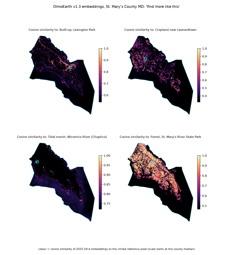
The first experiment is “find more like this.” I chose reference locations representing built-up land, cropland, tidal marsh, and forest. The script uses ESA WorldCover labels to locate a nearby consistent patch of the intended class, then averages a small neighborhood to form the reference vector. It compares that vector with every pixel in the county. The result is a continuous similarity surface. Values closer to one indicate a closer match in embedding space. This gives an analyst a way to explore where similar patterns occur before committing to a classification scheme.
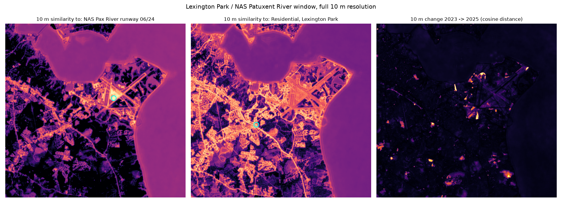
At 10 meters, the same approach produces recognizable patterns around Pax River and Lexington Park. A runway reference highlights paved areas, while a residential reference emphasizes much of the developed street pattern. The results also show why interpretation is important. Water receives a moderate similarity score in the runway example. The map alone does not explain which learned characteristics produced that match. A high similarity score gives us a candidate to examine, but it doesn’t establish that the candidate is another runway.
The second experiment adds labels. I aligned ESA WorldCover 2021 with the 40-meter grid and selected six classes: tree cover, grassland, cropland, built-up, water, and wetland. The script randomly samples 60 pixels per class, giving it 360 training examples. A logistic regression model then learns the relationship between those labels and the 2025 embedding vectors. This is a relatively small classification task because the embeddings already provide the input features.
The saved results show 94.5% agreement with WorldCover on the remaining eligible pixels. Grassland is the weakest class, with confusion involving cropland and built-up areas. The confusion matrix is useful because the overall percentage conceals those differences.
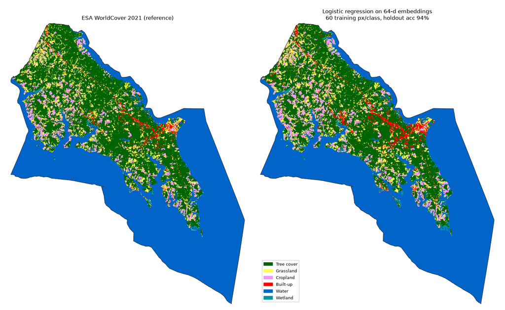
That percentage needs a precise description. The reference is a 2021 land-cover product, while the inputs represent 2025. Some disagreements may reflect actual change. The reference product also has its own errors, and the random sampling allows evaluation pixels to be close to training pixels. WorldCover also appears among OlmoEarth’s documented pretraining inputs, so this comparison should not be treated as validation against a wholly independent reference source.
I’d treat this as evidence that the embeddings support a useful local classification experiment. Establishing current land-cover accuracy would require independent reference observations and a more deliberate evaluation design, including geographic separation between training and test areas.
The third experiment compares each location with itself over time. After normalizing the vectors, the calculation is straightforward:
change = 1 - np.einsum("bhw,bhw->hw", embeddings_2023, embeddings_2025)
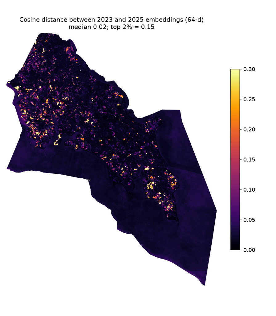
Here, the arrays contain normalized vectors arranged as bands, rows, and columns. Locations with similar representations in both years receive scores near zero. Larger values indicate greater differences. The notebook selects the strongest approximately two percent of county scores, groups connected pixels into polygons, and retains polygons covering at least one hectare. Those polygons are exported as GeoJSON and GeoParquet.
This is where the workflow starts to look very familiar. Once the candidates are geographic features, they can be intersected with parcels, compared with permits, summarized by watershed, or inspected against dated aerial imagery. The threshold is a screening choice. It identifies the strongest differences within this particular study area, but it doesn’t establish a universal boundary between changed and unchanged land. Agricultural cycles, vegetation conditions, and differences in observations can all complicate interpretation. Confirming construction, clearing, or another event requires additional evidence.
The notebook also includes a PCA visualization that reduces the 64 dimensions to three components and displays them as red, green, and blue. It provides another way to inspect spatial structure in the embeddings. The colors represent variation in the learned features, rather than natural color or named land-cover classes.
What interests me most about all of this is how readily the embeddings fit into existing geospatial practice. The inputs are arrays with geographic coordinates. The outputs are rasters, polygons, and attributes. The analytical choices remain familiar. You can select a resolution, align the reference data, define a sample, calculate a comparison, and inspect the result.
A natural extension would be to aggregate embeddings by parcel or another meaningful geography and store them alongside geometry and attributes in PostgreSQL. Similarity search could then become part of a broader query: find parcels with comparable embedding characteristics, within a specified area, subject to known land-use constraints. That would require testing how well aggregation preserves the patterns of interest, especially for mixed parcels. For now, this county example gives me a practical starting point. One set of precomputed embeddings supports several different questions, using tools that are already common in a geospatial Python environment. The next work is to examine individual candidates, bring in independent observations, and determine which of those questions the data can answer reliably. With all of that said, these results generally agreed with what I expected to see in this region.
OlmoEarth embeddings provide a reusable starting point for similarity search, classification, and change analysis, with the computational work of generating the representations already done. Distributing them through Source Cooperative makes that usefulness accessible. I can read the data directly into a local Python workflow, focus on an area of interest, and produce outputs that fit into familiar GIS tools. This is a small example, but it shows how much experimentation becomes possible when useful representations are published in a form that can be readily consumed.
